Deep Fade Kalman Filter Design

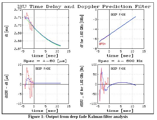
This example shows a SatLab plots for a design test of a Kalman filter to cope with time<br />delay and doppler during deep fade. These plots are from the period of maximum change in the rate of deep fade.
The script to generate these plots is shown below.
%demo Deep Fade Kalman Filter
%
% The requirements for handsets for GMPCS satellite systems is
% that they do not loose synchronization during short time
% deep fades. They need to include a filter to predict time
% delay and doppler during the time of a deep fade where
% synchronization signals are not received from a satellite.
% This filter needs to meet the requirements after receiving
% synchronization time delay and doppler synchronization
% data for a minimum specified time.
%
% In this demo a Kalman filter is designed and analyzed
% that easily meets the requirements to predict dt and df
% for 128 frames after receiving synchronization data from
% a satellite for 48 frames, with associated measurement
% errors. The results are for the time of maximum rate of
% change of df.
%
% The Kalman Filter also smoothes DTOA and DFOA for the ISU
% SatLab demo: Horst C. Salzwedel

help demoDeepFadeKF

% Initialization
removeAll;
clearGraphic();
clear;

% L-band frame length = 90 ms
LBframe = .090;

% L-band frequency
fLB = 1.62e9;

% time constant tau = 600 seconds
tau = 1200;

% standard deviations
rand("normal");       % set random number generator to 'normal'
rand("seed", 260342); % set seed for repeatability of results

sigdtm  = 4e-6;       % measurement error 4 microseconds
sigdfm  = 20;         % measurement error 20 Hz
sigdtr  = 2e-6;       % reporting error 2 microseconds
sigdfr  = 9.8;        % reporting error 9.8 Hz
siga    = 5e-5;
sigDTOA = sigdtm + sigdtr;
sigDFOA = sigdfm + sigdfr;

% state distribution matrix
A = [0 1 0
     0 0 1
     0 0 -1/tau];

B = [0
     0
     1];

% output matrix
C = [1/cLight  0           0 
     0         fLB/cLight  0];

% continous to discrete conversion
[Phi, Gam] = c2d(A, B, LBframe);
Q          = siga;

% initialization
loadreplaceAll("./IRsingle.data");
setSimEpoch(2002,3,26,11,58,54.91185); % 0 sec
setSimTime(0);
g    = GeoPosition(3);
g    = g(1:2,:);
lat0 = g(1, 1);
lon0 = g(2, 1);

setStationParameter('E1', I_earth, 0, lat0*r2d, lon0*r2d, 0);
setSimEpoch(2002,3,26,11,58,34.91185); % -20 sec
setSimTime(0);
setSimStepSize(LBframe);

% initialization of ISU
[d, r, a, e, v] = RelPosition('E1');
dfISU0 = r(2)/cLight*fLB;
dfISU  = dfISU0;
dtISU0 = d(2)/cLight;
dtISU  = dtISU0;

% state vector
x = [dtISU*cLight dfISU*cLight/fLB 0];
P = diag([1e1 1e-6 1e-2]);

% covariance matrix R
R = [sigDTOA^2   0
     0           .8*sigDFOA^2];

% initialization of SV
j     = 0;
iSV   = 0;
dtsum = 0;     % summer for dt averaging
dfsum = 0;     % summer for df averaging
DTOA  = 0;     % SV time delay error measurement
DFOA  = 0;     % SV doppler frequency error measurement
ii    = [-47:127];

for i = ii,
    iSV = iSV + 1;
    j = j + 1;
    stepSim;   % step simulation forward by 1 L-band frame

    %predict time delay and doppler frequency
    x = Phi*x; % Kalman Filter time update
    y = C*x;
    dtISU = y(1);
    dfISU = y(2);
    
    % Doppler and time delay of up/down link
    [d, r, a, e, v] = RelPosition('E1');
    Mdf(j) = r(2)/cLight*fLB;      % store true df in array for plotting
    Mdt(j) = d(2)/cLight;          % store true dt in array for plotting

    % measurement of dt and df by SV
    dtsum = dtsum - dtISU + Mdt(j) + sigdtm*rand(1);
    dfsum = dfsum - dfISU + Mdf(j) + sigdfm*rand(1);
    % measurement update
    if (iSV == 4)
        DTOA   = dtsum/4 + sigdtr*rand(1);
        DFOA   = dfsum/4 + sigdfr*rand(1);
        dtsum  = 0;
        dfsum  = 0;
        iSV    = 0;
        dtISUm = DTOA;
        dfISUm = DFOA;
        if i < 0, % time before fade
            y_m = [DTOA
            DFOA]; % measurements from satellite
            M = Phi*P*Phi` + Gam*Q*Gam`;  % error covariance time update
            K = M*C`*inv(C*M*C` + R);     % Kalman filter gain
            x = x + K*(y_m);              % measurement update
            P = M - K*C*M;                % error covariance measurement
            
            update
            imeasurement = j;
        endif
    endif % 4th frame

    MdtISU(j) = dtISU+DTOA;
    MdfISU(j) = dfISU+DFOA;

    % estimate y
    y_e = C*x;
    EdtISU(j) = y_e(1);
    EdfISU(j) = y_e(2);
endfor
erase

title('ISU Time Delay and Doppler Prediction Filter')

window('221')
iim=ii(1:imeasurement);
plot(ii`*LBframe, Mdt*1e3, 'green',
     iim`*LBframe, MdtISU(1:imeasurement)*1e3, 'red',
     ii`*LBframe, EdtISU*1e3, 'blue', 'grid')
xlabel('time [sec]');
ylabel('dt [ms]');
wtext(1,2.645,'Deep Fade')
wtext(-4,2.622,'DTOA','red')

window('223')
plot(ii`*LBframe, (EdtISU - Mdt)*1e6, 'grid', 'blue',
     iim`*LBframe, (MdtISU(1:imeasurement) - Mdt(1:imeasurement))*1e6,
     'red');
xlabel('time [sec]');
ylabel('dtISU - dt (ms)',
       'll ll sgls');
title(' Spec = +-60 (ms) ',
      ' lll sgls ')
wtext(1,8,'Deep Fade')

window('222')
plot(ii`*LBframe, Mdf/1000, 'grid', 'green',
     iim`*LBframe, MdfISU(1:imeasurement)/1000, 'red',
     ii`*LBframe, EdfISU/1000, 'blue');
xlabel('time [sec]');
ylabel('df for 1.62 GHz [KHz]');
wtext(1,-1,'Deep Fade')
wtext(-4,-7,'DFOA','red')

window('224')
plot(ii`*LBframe, (EdfISU - Mdf), 'grid', 'blue',
     iim`*LBframe, (MdfISU(1:imeasurement) - Mdf(1:imeasurement)),
     'red');
xlabel('time [sec]');
ylabel('dfISU - df for 1.62 GHz [Hz]');
title(' Spec = +- 600 Hz ',
      ' lll l ')
wtext(1,80,'Deep Fade')
MLDesign Technologies, Inc.

Mainnavigation

Subnavigation

BORDER

Pagecontent

Deep Fade Kalman Filter Design
